An introduction to Spatial Databases

Foreword

This post is a perpetual work in progress and a may decide to update it in future. The version below was written at the beginning of March 20, right before the beginning of the COVID lockdown in Italy. Although maybe incomplete, I decided to publish it. Given current trends (20k new infected yesterday) another lockdown may arrive soon.

1 Introduction

1.1 Motivation

Cyber-physical systems are characterized by a continuous interaction with the real world, from which data are gathered and counteractions may be taken, either using actuators or indirectly by human operators. Situational information, i.e. context, related to collected data, captures domain-specific aspects of the monitored phenomena. Location is one of such kind. Spatial databases are optimized for storing and querying data defined in a geometric space, by providing for the representation of both geometric and topological entities, as well as their efficient retrieval and processing, by adding specific indexes.

1.2 Summary

The aim of this post is to provide the reader with a primer into spatial data management and analysis. In the first part, foundations of spatial data management will be provided, namely the following will be described: spatial data types, reference systems and indexes, as well as common data formats.

Throughout this introduction, we will be adopting open source solutions: the postgres DBMS and its extensions PostGIS and pgrouting, as well as the Desktop tool QGIS. For the avid programmers we will be also mentioning common Python libraries for Spatial data processing. 

2. Spatial Databases

Spatial databases are designed to provide efficient organization, storage and retrieval of spatial objects, i.e. entities that embed spatial attributes such as location and altitude and can be efficiently related in spatial terms, e.g. in terms of distance or more sophisticated polygon containment. 

2.1 PostGIS

Throughout this introduction we will be referring to PostGIS a widely used and open-source (GPL v.2) spatial extension for the PostgreSQL database management system (BSD-licensed). PostGIS conforms to the Open Geospatial Consortium (OGC) standards and as such it is a sort of lingua franca for Spatial Databases. Although there exists several solutions, such as Spatial Lite, Oracle Spatial and ESRI’s ArcGIS, the OGC consortium standardizes how geographic data is organized and accessed, so learning PostGIS functionalities is one of the best ways to get acquainted with geographical information systems (GIS).

2.2 Spatial Data Types

PostGIS distinguishes data types in the following categories:

• Geometry, a 2D representation of space allowing for basic Geometrical calculus

• Geography, a spheroidal representation, i.e. locations consider the earth’s curvature

• Raster, a bitmap representation, i.e. a matrix of values from a reference palette

• Topology, a network representation, i.e. a graph whose edges can be associated with additional attributes, for instance to allow for the resolution of routing problems;

The geometry data types relates to a Cartesian planar space, whereas the geography types assume a geodetic coordinate system, i.e., the WGS 84 lon/lat SRID 4326, which considers the earth’s curvature.

The Raster and Topology types will be discussed more thoroughly in Sect. and Sect respectively. The geometry and geography data types are placeholders for different reference systems, either planar or geodetic types, thus it is with the respective subtypes that data are actually characterized. Those subtypes, called type modifiers, are more specific and can be related as long as they share the same spatial reference system (SRID). We will discuss reference systems in the next Sect. 2.2.

Type modifiers include:

• point - coordinate point

• POINT - 2D point (x, y)

• POINTZ - 3D point (x, y, z)

• POINTM - 2D point and measured value (x, y, m)

• POINTZM - 3D point and measured value (x, y, z, m)

• linestrings - connected straight line segments

• LINESTRING - 2D sequence of POINT elements

• LINESTRINGZ - 3D sequence of POINTZ

• LINESTRINGM - 2D sequence of POINTM

• LINESTRINGZM - 3D sequence of POINTZM

• polygons - enclosed shapes whose perimeter is a linestring

• POLYGON - closed shape delimited by a linestring

• MULTIPOLYGON - collection of polygons

• collections of geometries

• MULTIPOINT - multiple independent points

• MULTILINESTRING - collection of linestrings

• MULTIPOLYGON - collection of polygons

• GEOMETRYCOLLECTION - collection of heterogeneous geometries

• polyhedrons

• POLYHEDRALSURFACE - multiple polygons sharing edges and constituting a polyhedron

• curves

• CIRCULARSTRING - sequence of arcs, each delimited by a pair of points

• COMPOUNDCURVES - collection of circular strings and linestrings

• CURVEDPOLYGON - polygon 

2.3 Reference Systems

A spatial reference system is an unambiguous coordinate system that is generally agreed to project spatial entities. Each reference system is a model of the earth, i.e. a simplified representation capturing specific aspects. Historically, we distinguish in the following models:

• ellipsoid and spheroid - a 3D ellipse model described by a polar and an equatorial radii

• geoid - following the heterogeneous orography of the earth different gravity measures are taken (e.g. at different locations having different elevations)

2.4 Data Formats

Standard spatial data formats allow for the interoperation of multiple components as a combined system. PostGIS supports the following formats:

• WKB/WKT - Well-known binary and Well-known text - respectively binary and text formats to represent geometry data on a map.

• KML - Keyhole Markup Language - XML-based format for spatial data

• GML - Geography Markup Language - XML-based format for spatial data

• GeoJSON - Geometry JavaScript Object Notation - A Spatial variant of the JSON, typically used for consumption in web services

• SVG - Scalable Vector Graphics - a vectorial graphics format

• X3D - Extensible 3D Graphics - XML-based format 

2.5 Raster formats

Rasters are matrix formats. PostGIS supports 2D matrices, which can be georeferenced, i.e. related to a reference system so that operations on the raster can be mapped to other representations used to organize the data. Rasters can be created from geometries using ST_AsRaster, created as manipulation from other rasters or else imported with utilities such as raster2pgsql.

3. Functionalities

3.1 Geometry relationships

Geometries are generally enclosed by a bounding box, which is used for geometry relationships since spatial search based on bounding boxes can be performed efficiently and quickly. Accordingly, the coordinates of objects’ bounding boxes can be pre-calculated and stored in indices that can be queried efficiently. As such, geometry operators are commonly used to reduce the size of the search space in spatial terms, before performing more accurate searches, for instance with geography operators.

Specifically, we distinguish the following geometry binary operators (i.e. A op B):

• && - 2D bounding box intersection of B

• &&& - 3D bounding box intersection of B

• &< - 2D bounding box overlaps or left of B

• &<| - 2D bounding box overlaps or below of B

• &> - 2D bounding box overlaps or right of B

• << - 2D bounding box strictly left of B

• <<| - 2D bounding box strictly below of B

• = - 2D bounding box same bounding box of B

• >> - 2D bounding box strictly right of  B

• @ - 2D bounding box contained by B

• |&> - 2D bounding box overlaps or above of B

• |>> - 2D bounding box strictly above of B

• ~-  - 2D bounding box contains the one of B

3.2 Distance operators and KNN

Distance operators are used for proximity analyses, i.e. those cases in which we study distances between objects. 

PostGIS has two main distance operators:

• ST_DWithin(A, ref, max_distance) returns true for those object pairs falling within a certain distance and can be as such used within WHERE clauses to select those object away within a certain distance

• ST_Distance(A, ref) returns the distance between two objects 

Distance operators can be applied to both geometry and geography data. Mind that, geometry and geography operators will act on different models, thus returning results of different accuracy and under different performance.  A common solution is to reduce the result set by applying faster k-NN operators (since they use the bounding box distance) and then apply the more costly distance operators on the smaller set to get an exact result.

For geometry types we distinguish in the following k-NN distance operators:

• <#> returning the minimum distance between the bounding boxes of two objects

• <-> returning the bounding box centroid distance

Contrarily to the operators seen in 3.2, those operators do not use spatial indexes when used in where and join clauses and do use a spatial index only in an order by clause. 

Since k-NN operators only work with geometry data, a common solution is to firstly convert geography data to geometry, perform the necessary computation, and finally convert back the result to a geography. 

3.3 Mapping functionalities

In this section, we discuss a number of functionalities that have common application on geographic information systems:

• geotagging - is the technique by which entities such as geometries or points can be associated to the entity that contains them, for instance a region or a state, as well as close landmarks or points of interests; we distinguish respectively in

• region tagging - a geometry is tagged with the region (read geometry) that contains it; Examples are the function ST_Intersect and ST_Contains.

• linear referencing - a point is tagged with the point in the closest point within a linestring (e.g. street segments). A common case is the snapping of GPS readings to the closest street (i.e. linestring). Given a point and a linestring, the function ST_LineLocatePoint returns a value between 0 and 1 to identify the location on the linestring that is closest to the reference point. This value can then be used to generate an actual point on the line (i.e. ST_LineInterpolatePoint) or to create a segment within the original linestring (i.e. ST_LineSubstring). A more general function ST_ClosestPoint can return the closest point on a generic geometry, thus it is not limited to neither points nor linestrings. Let’s suppose we want to locate the closest point on a street for a GPS reading. We would then start with i) ST_DWithin to narrow the search space within a certain distance from the point (i.e. the GPS error), ii) use ST_ClosestPoint to find the closest point placed on one of those geometries nearby and iii) finally order them by ST_Distance to retrieve the closest geometry.

• geocoding - is the problem of converting street text representation into the geographical position, e.g. lat/lon or point in space, usually referred to the street centerline. Reverse geocoding converts back spatial coordinates into street addresses. PostGIS includes the TIGER geocoder component which can be installed as an extension.

• geohashing -  is a lossy coding technique allowing for converting lat/lon coordinates into a hash string that can be used to more easily organize spatial information (e.g. across distributed systems). PostGIS has a ST_GeoHash function performing the conversion.

4. Indexes

Traditional data types, such as strings and numerics, rely on B-tree variants to build range indexes. On the contrary, PostGIS provides the generalized search tree (GIST) and generalized inverted tree (GIN).

5. Topology data

In this Section we introduce pgRouting, a PostgreSQL extension for developing graph analysis and routing applications. A common use is to find the shortest route in a road network. In this case, the first step is to build a topology out of a table of linestring roads, by calling the pgr_createTopology function (e.g. as a select from the original table). The function iterates over the table to assign each node a unique identifier. The result is a target edge table and a vertices table called like the edge table plus a suffix _vertices_pgr. In addition, a weight or cost can be assigned to each edge, for instance based on the segment length (see ST_Length) or use-case-specific factors. Graph algorithms, such as Dijkstra, can then be applied to traverse the graph and find the cost-minimizing path between one and multiple nodes, as well as find sequences of nodes (i.e. an itinerary) minimizing the total distance, as in the traveling-salesman problem (see pgr_tsp function). Please see an example analysis here.

6. Playing with Postgis and PGRouting

6.1 Setup

6.1.1 Starting from a Postgis docker container

To show how postgis can be set up, we prepared here a very simple docker container installing Postgres and Postgis, and finally importing Italy as pbf file from the openstreetmap (OSM) project. Please have a look at the Docker documentation for how to build and start docker containers. In general, a "docker build --tag tagname:version ." from the project folder will be enough to build, while a "docker run -rm -p 50432:5432 tagname:version" will be enough to get an up and running postgis container. 

As visible in the Dockerfile, after setting up postgres and enabling postgis the tool osm2pgsql imports the pbf file directly in the DB:

osm2pgsql --slim -C 18000 --number-processes 8 --host localhost --port 5432 \

--database $DBNAME --username $POSTGRES_USER mapfile.pbf

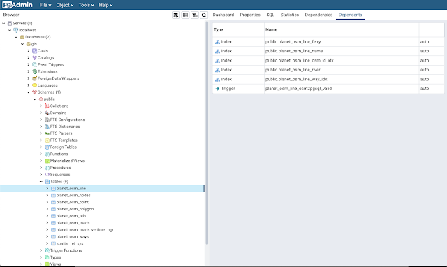
To explore the DB structure you can connect to port 5432 using the pgAdmin official client. 

General-purpose DB clients, such as DBeaver and DataGrip shall similarly also be used.

Alternatively, you may use the open source quantum-GIS (QGIS) to explore the underlying map representation stored in the DB.

6.1.2 Starting from a pg-routing docker container

To explore pg-routing, we extended the pgrouting/pgrouting docker image into a new image available on this github repo. The build process uses a multi-stage build starting with a java jdk where the osm2po tool is downloaded and used to convert the pbf file of a target osm map of choice (in the example we set it to Iceland given its small size). The output of osm2po is an sql file, which is then imported in the following docker build stage inheriting from the pgrouting/pgrouting. Moreover, we use tini as docker entrypoint and introduce the entrypoint.sh to wrap the existing docker-entrypoint.sh (inherited from the postgis image) to start postgres, then run a number of queries to prepare the db: i) to enable the postgis and pgrouting extensions, ii) import the osm_2po_4pgr.sql file, and iii) create the vertices table; The osm2pgsql tool may also be used to import additional osm info, for instance to enrich routes with road segment information (e.g. speed limits). The process finally waits for all the started processes to complete and return.

We can now connect to the running instance from QGis:

QGIS view of the routable map of Reykjavik - Iceland

Alternatively, we can run graph algorithms, such as Dijkstra's, using a postgres client, such as pgAdmin:

The result is a route from Kringlan to Listabraut:

| seq   | node  | street       | cost   | dist_m |
|-------|-------|--------------|--------|--------|
| 1     | 15541 | "Kringlan"   | 0.0021 | 105.96 |
| 2     | 14187 | "Kringlan"   | 0.0006 | 136.71 |
| 3     | 14221 | "Kringlan"   | 0.0010 | 187.09 |
| 4     | 14183 | "Kringlan"   | 0.0004 | 208.99 |
| 5     | 14202 | "Kringlan"   | 0.0003 | 225.85 |
| 6     | 8202  | "Kringlan"   | 0.0006 | 257.12 |
| 7     | 15078 | "Kringlan"   | 0.0006 | 285.48 |
| 8     | 44099 | "Kringlan"   | 0.0001 | 290.65 |
| 9     | 949   | "Kringlan"   | 0.0003 | 307.10 |
| 10    | 44104 | "Listabraut" | 0.0011 | 361.32 |
| 11    | 59469 | "Listabraut" | 0.0011 | 415.17 |
| 12    | 5798  | "Listabraut" | 0.0006 | 447.32 |
| 13    | 19378 | "Listabraut" | 0.0005 | 470.70 |
| 14    | 44107 | "Listabraut" | 0.0001 | 476.48 |
| 15    | 16558 | "Listabraut" | 0.0001 | 480.31 |
| 16    | 16555 | "Kringlan"   | 0.0002 | 488.81 |
| 17    | 44108 | "Listabraut" | 0.0002 | 498.14 |
| 18    | 44109 |              | 0.0000 | 498.14 |

6.1.3 Starting from a full-fledged docker container for tile serving

To explore the full potentiality of the OSM maps on postgis, we extended the overv/openstreetmap-tile-server docker image to also import pgrouting topologies. Once built, the container can be run to import any of the OSM pbf files, either previously downloaded to a folder mounted as volume or directly downloaded by the container:

docker run \
    -e UPDATES=enabled \
    -v /absolute/path/to/luxembourg.osm.pbf:/data.osm.pbf \
    -v /absolute/path/to/luxembourg.poly:/data.poly \
    -v openstreetmap-data:/var/lib/postgresql/12/main \
    overv/openstreetmap-tile-server \
    import

docker run \
    -e DOWNLOAD_PBF=https://download.geofabrik.de/europe/luxembourg-latest.osm.pbf \
    -e DOWNLOAD_POLY=https://download.geofabrik.de/europe/luxembourg.poly \
    -v openstreetmap-data:/var/lib/postgresql/12/main \
    overv/openstreetmap-tile-server \
    import

The run.sh script is the docker entrypoint. When passing import the DB is set up similarly to the one described in the previous Sect. 6.1.2, i.e. by enabling desired extensions and finally calling osm2pgsql to import the osm file. Check the line here. There are various ways to import pgrouting data. One is to use the osm2pgrouting import tool. An alternative is to use osmconvert to convert the pbf file to osm and then use the osm2po to import the osm data and make it directly routable. This FOSS4G workshop provides a complete tutorial using pgrouting. Sect. 12.1 shows how a routable network topology for pgrouting can be derived from data previously loaded with osm2pgsql. Specifically, planet_osm_roads already provides road information, such as link id (gid), name (name) and geometry (the_geom), which allows us for displaying it as layer in QGIS, as follows:

The network is however currently non-routable. An additional step is required, i.e. a call to the pgr_createTopology function to build a network topology from geometry information.

In detail, the source and target columns are added to the planet_osm_roads table and a "SELECT pgr_createTopology('planet_osm_roads', 0.00001, 'way', 'osm_id');" is run.  A new table named planet_osm_roads_vertices_pgr was now added.  The source and target columns in planet_osm_roads correspond to an id in the planet_osm_roads_vertices_pgr table.

Simple routing analyses can be performed, for instance:

SELECT * FROM pgr_dijkstra('

    SELECT osm_id AS id,

         source,

         target,

         cost_minutes AS cost

        FROM planet_osm_roads',

    13224, 6549, directed := false);

Please note that the pgRoutingLayer plugin for QGIS may also be handy for routing analyses.

Once the import process is done, the container can be run as follows:

docker run \
    -p 8088:80 \
    -p 50432:5432 \
    -e PGPASSWORD=secret \
    -v openstreetmap-data:/var/lib/postgresql/12/main \
    -d overv/openstreetmap-tile-server \
    run

A leaflet demo is now available at http://localhost:8088/tile/{z}/{x}/{y}.png to query the tile server.

This should also provide an extendable starting point to develop web applications with Leaflet. 

Bibliography

1. Regina O. Obe and Leo S. Hsu. 2015. PostGIS in Action (2nd. ed.). Manning Publications Co., USA.

2. Regina O. Obe, Leo S. Hsu, and Gary E. Sherman. 2017. PgRouting: A Practical Guide. Locate Press, Chugiak, AK.